Brock Algebra using k-values

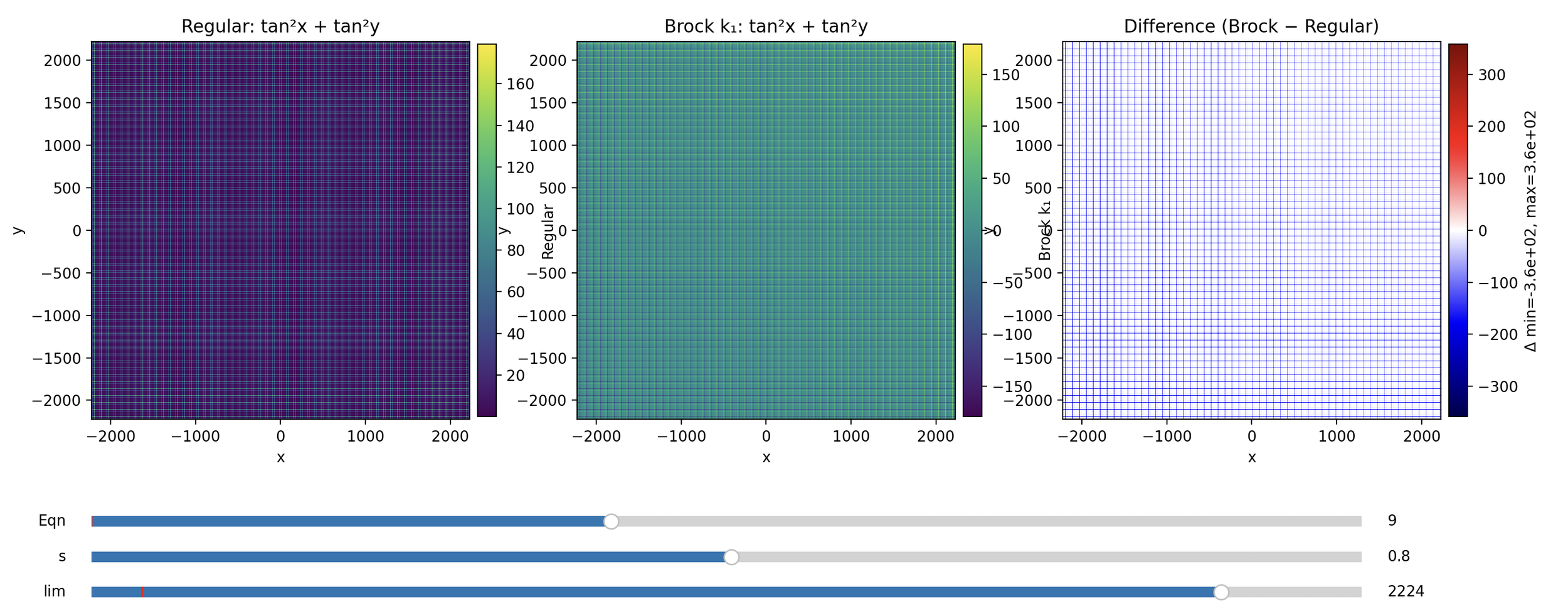
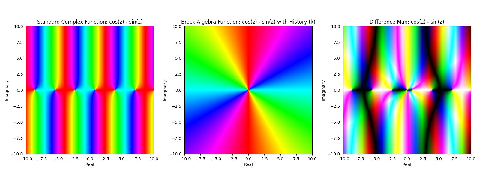
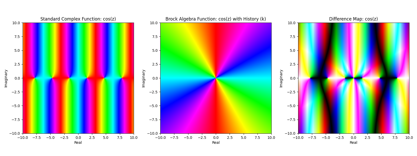
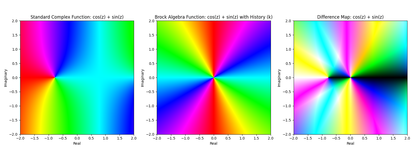
z = cos(x)+ cos(y)

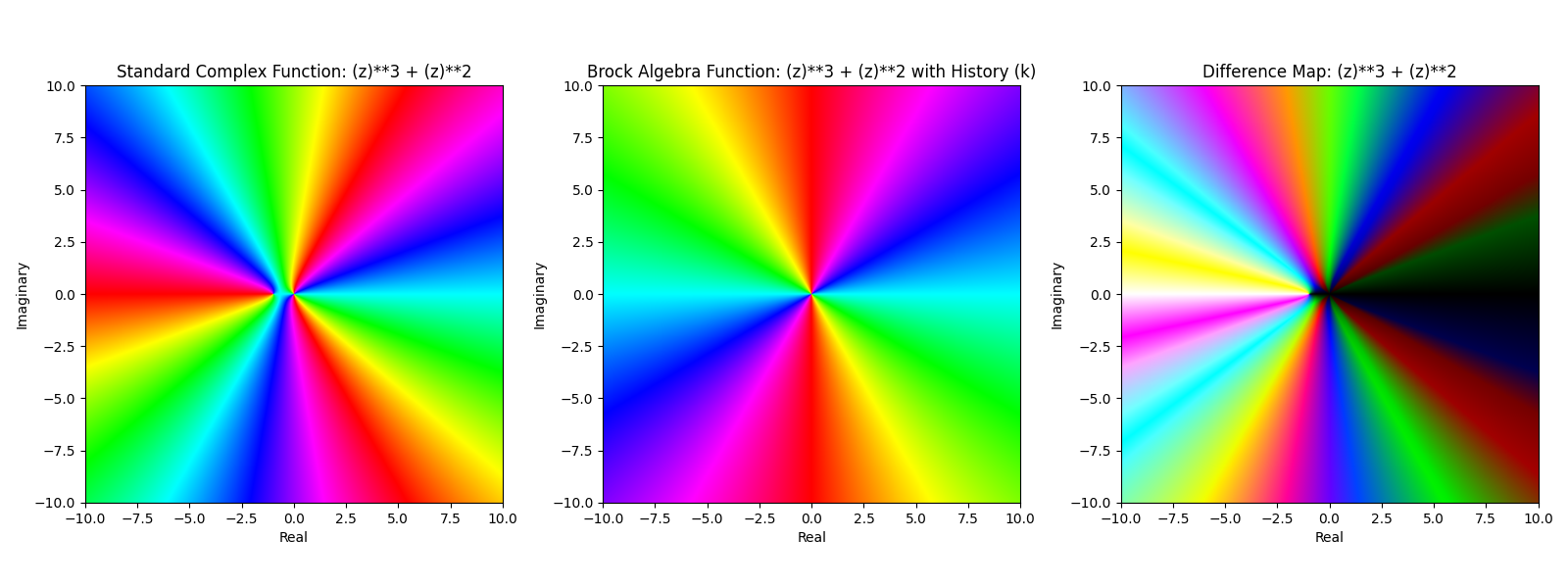
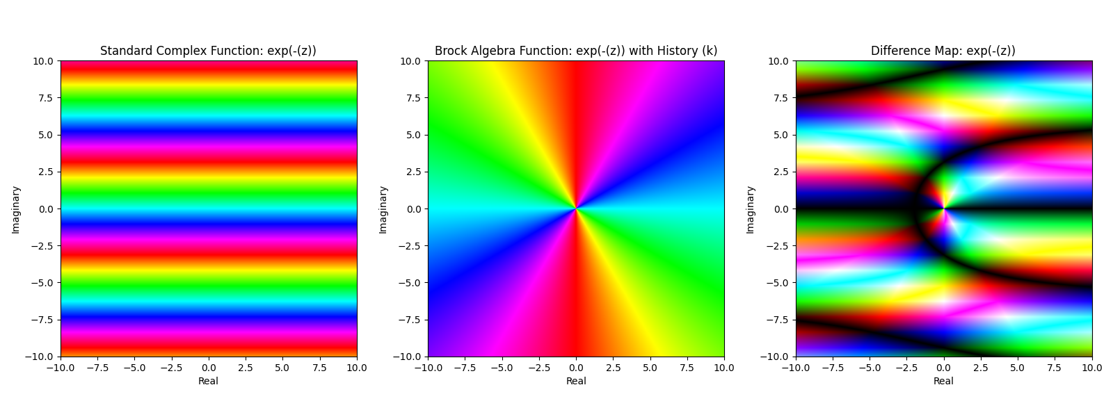
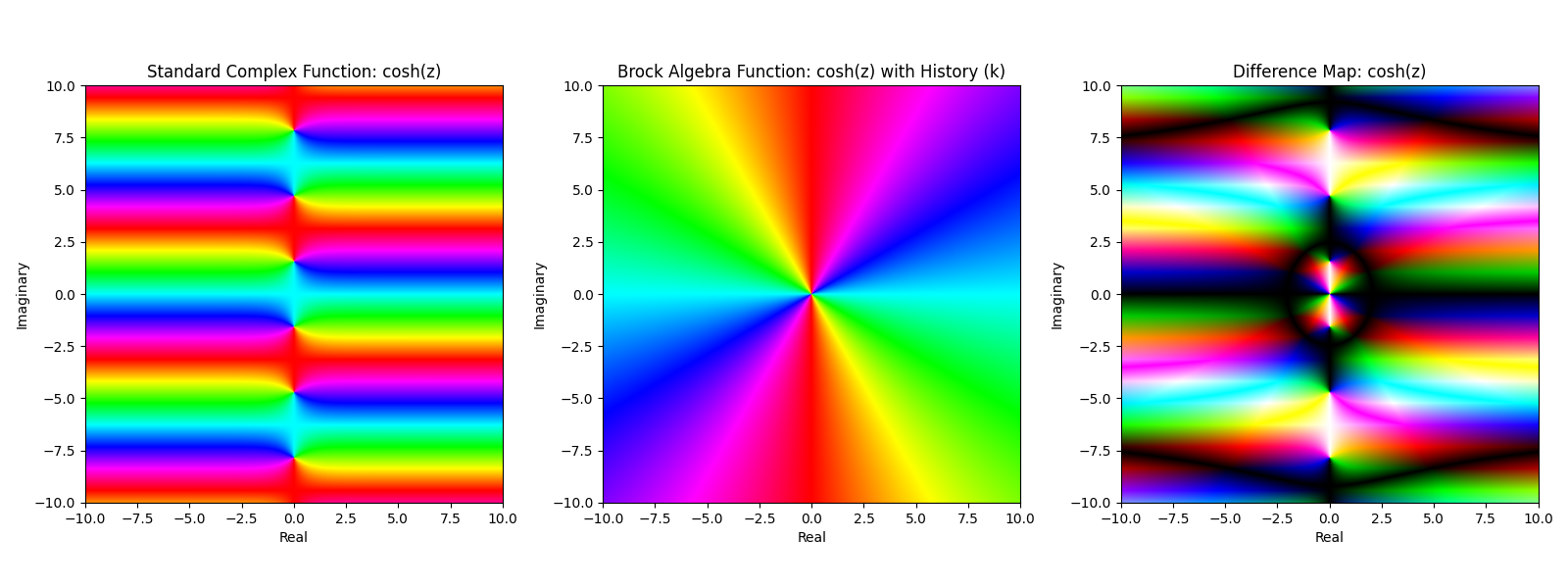
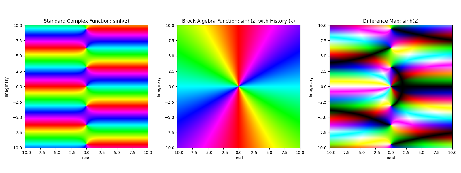
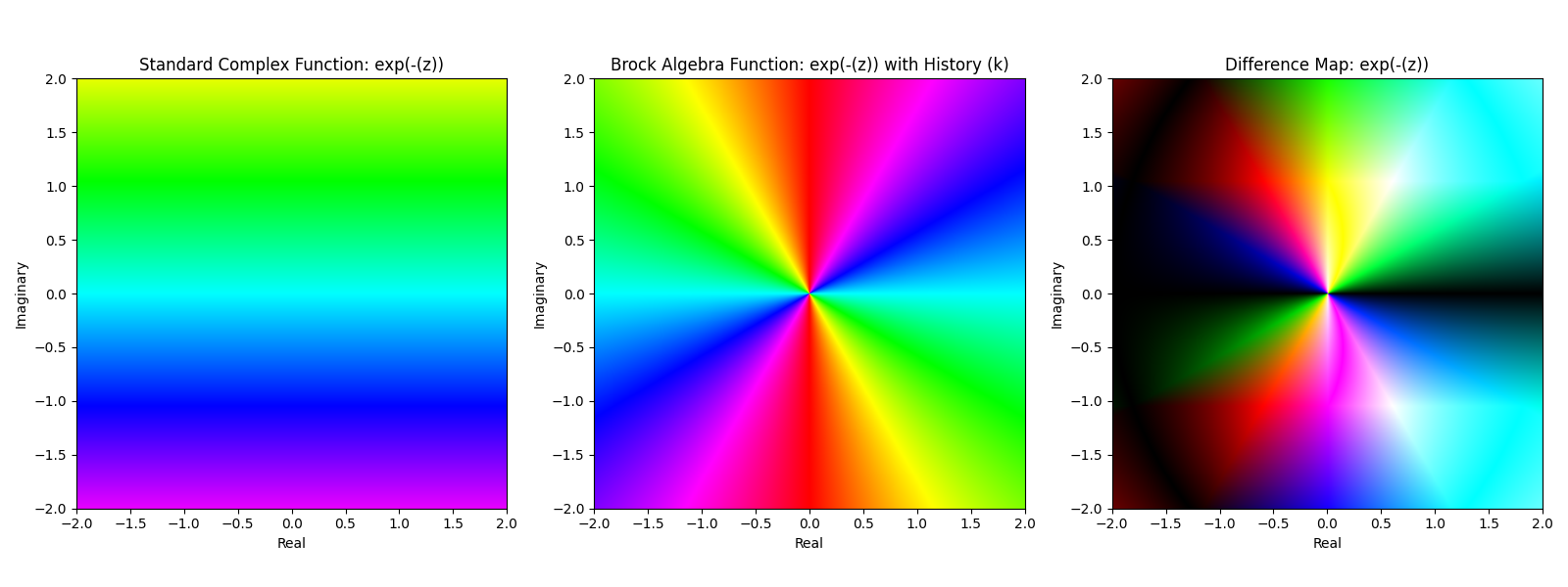
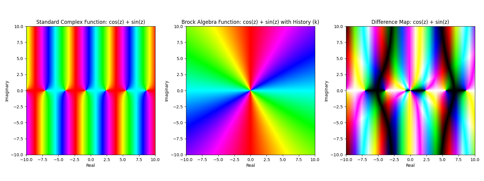
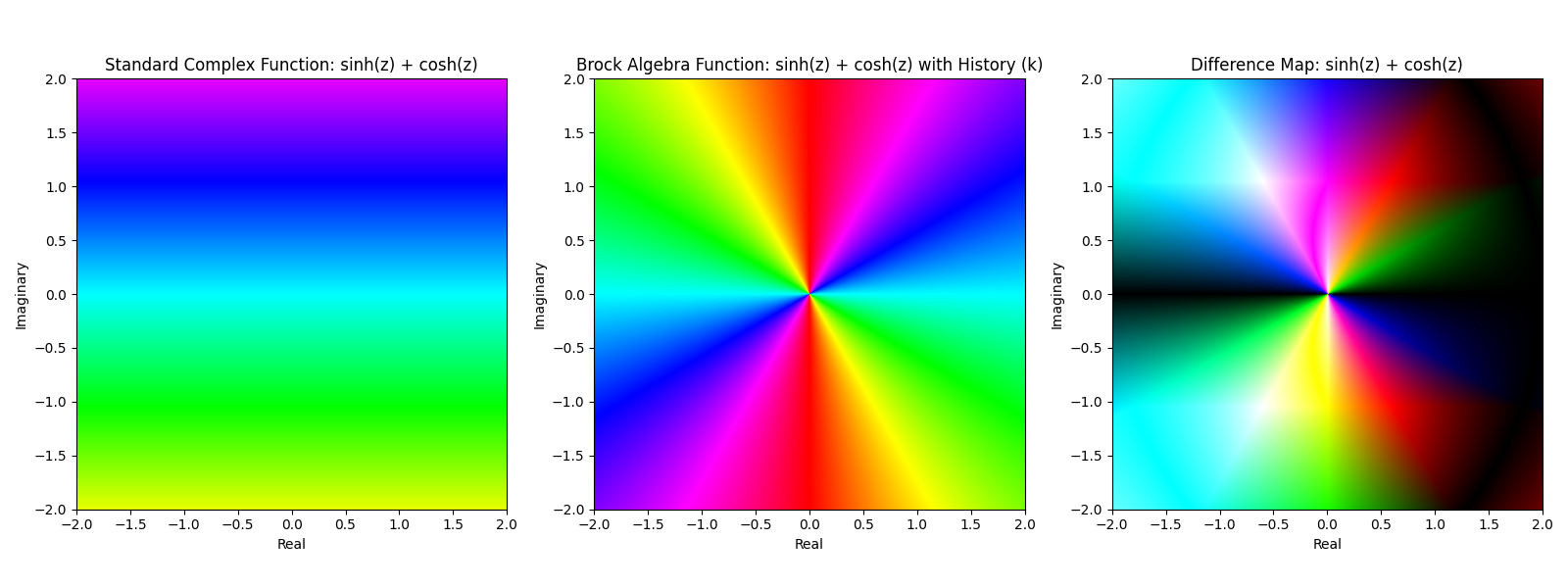
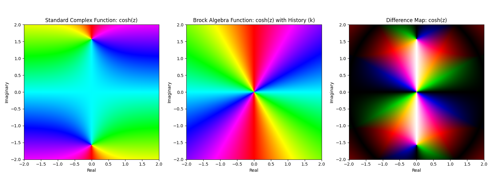
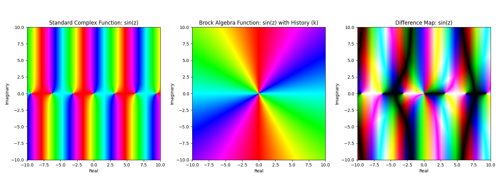
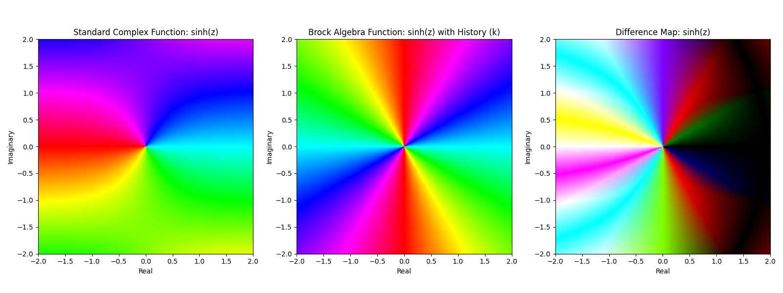
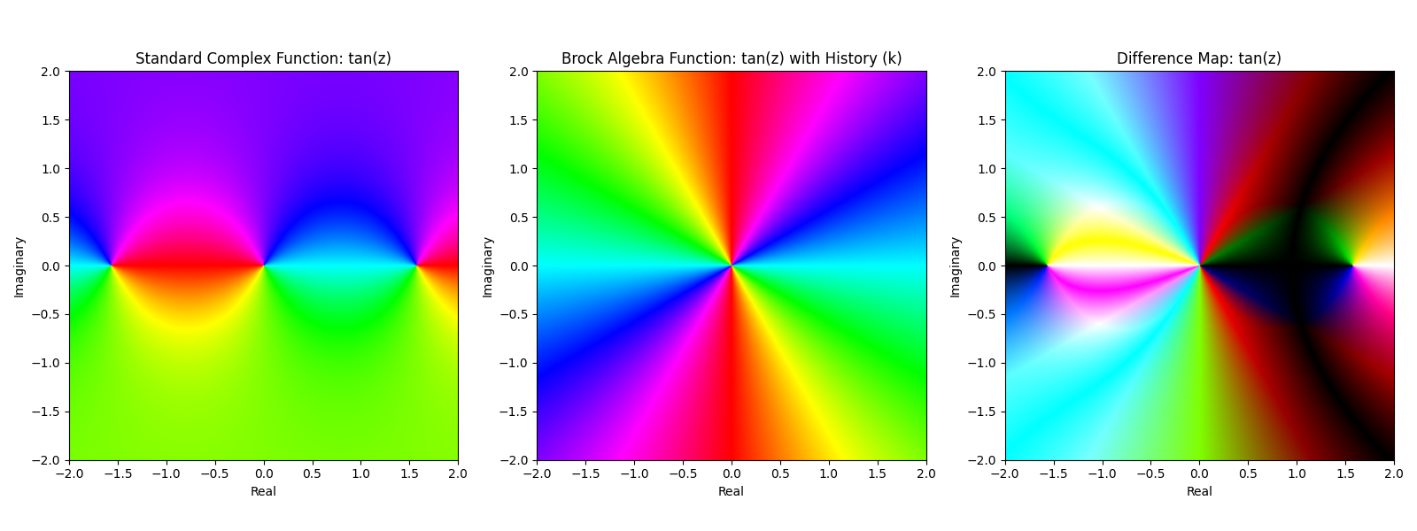
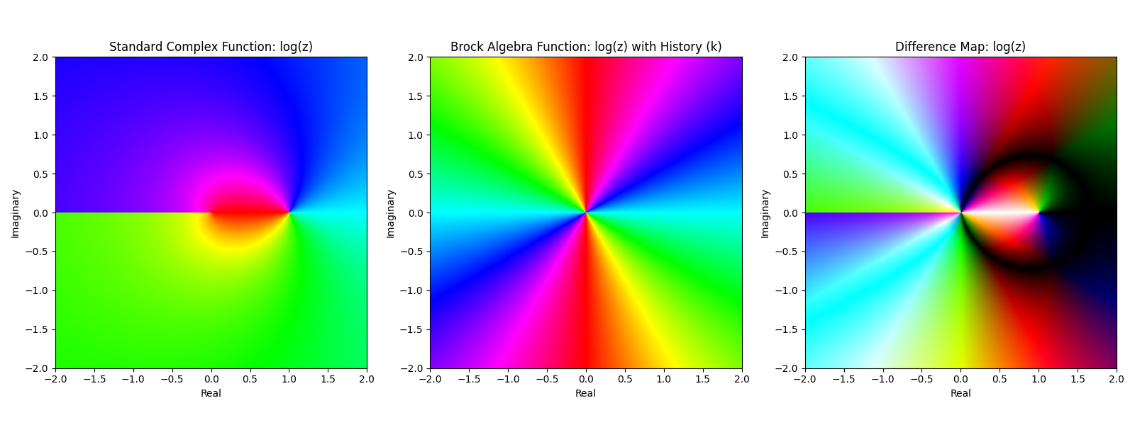
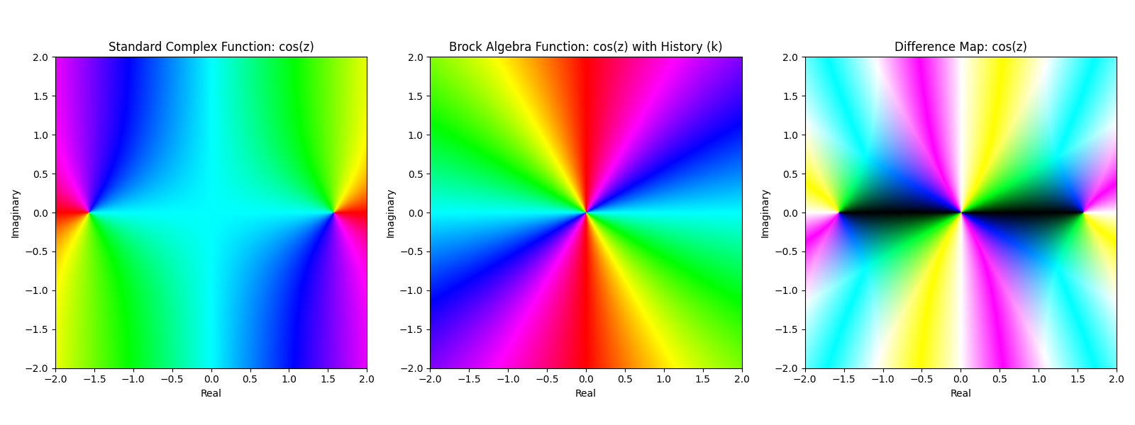
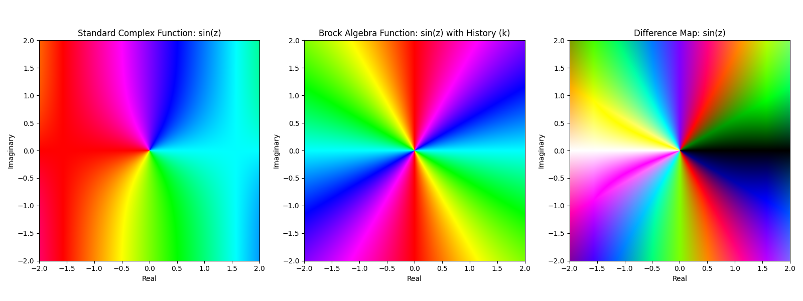
Shown regularly and then under Brock Algebra(k₁)
Followed by a difference map

Brock Algebra - Sign preservation using k-values

Introduction

Brock Algebra is an experimental extension of classical algebra that augments each number with a history component, allowing us to trace operations in ways that standard arithmetic does not. One compelling variant is Brock Algebra k₁, in which any exponentiation – especially squaring – preserves the original sign rather than collapsing negatives to nonnegative outputs. In this article we will:

1. Recall the core k-value intuition and practical uses
2. Define operations in full Unicode math
3. Explore special cases kₙ, k₂, k₁, and k₀
4. Fix our sign-representation choice once and for all
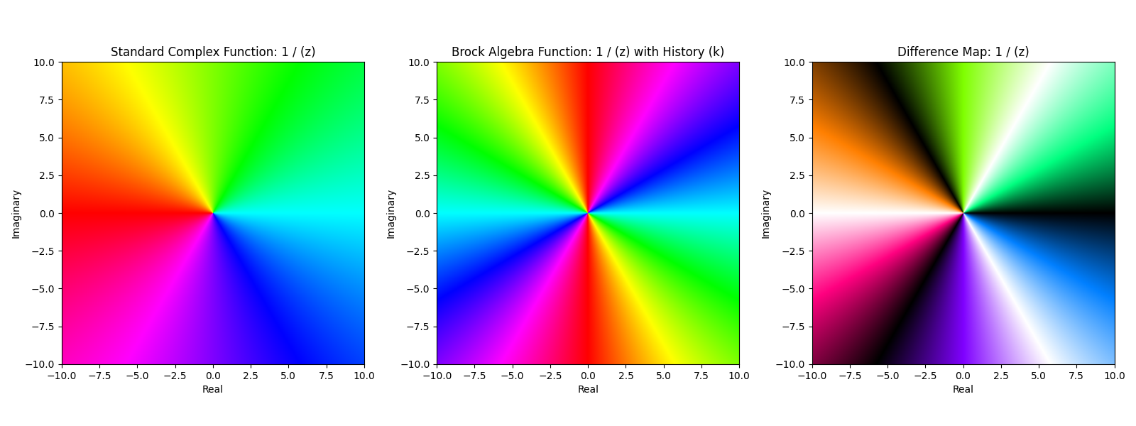
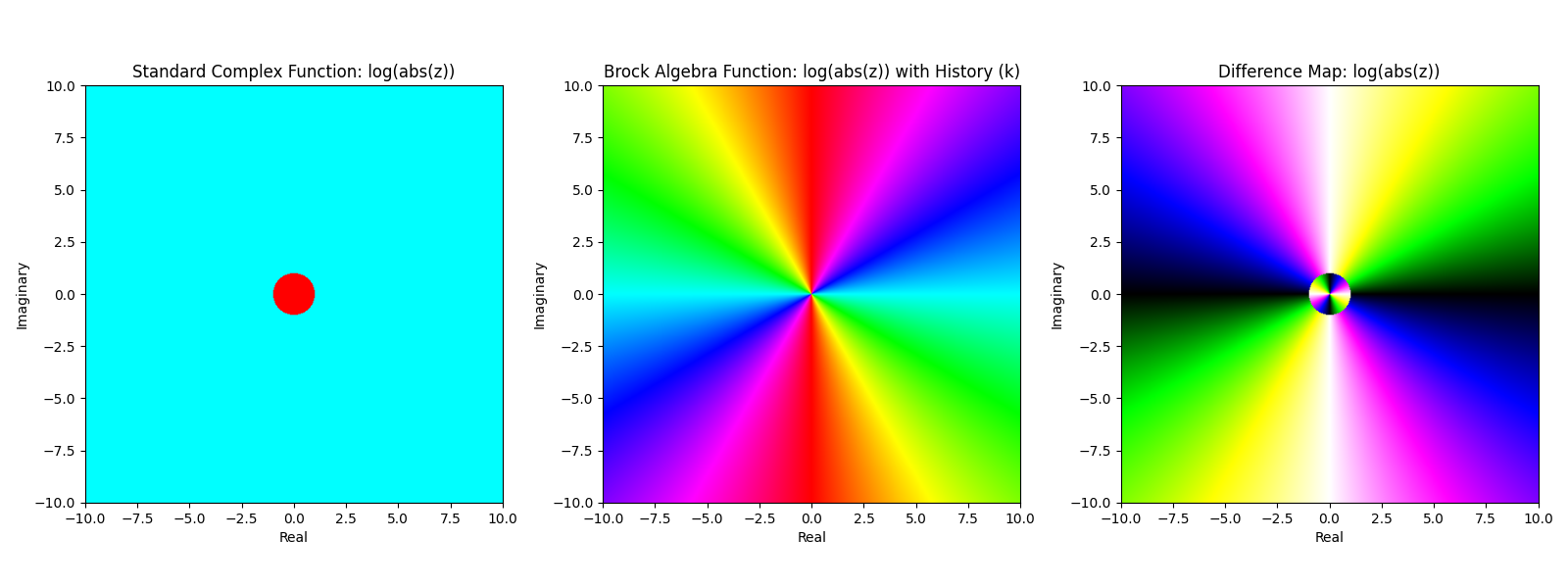
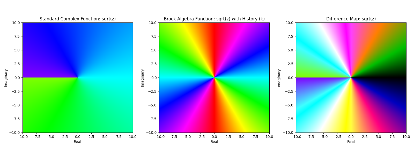
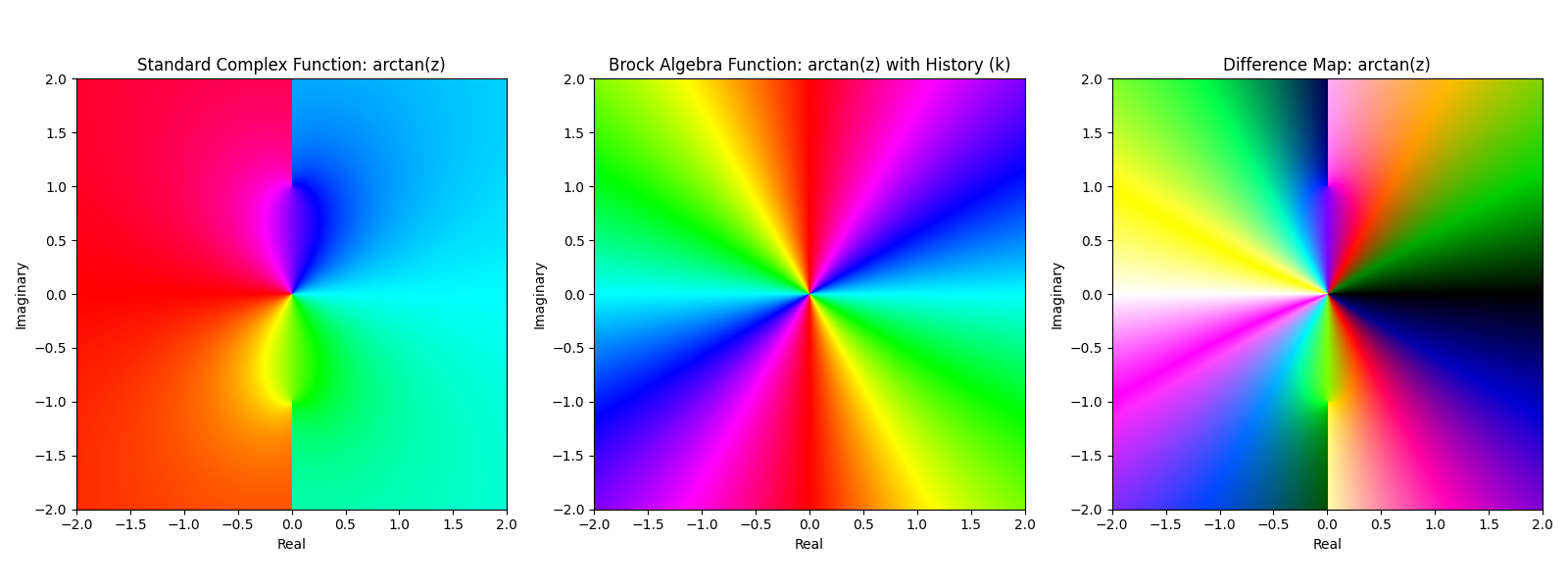
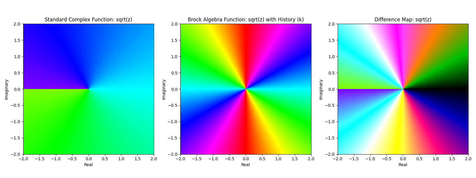
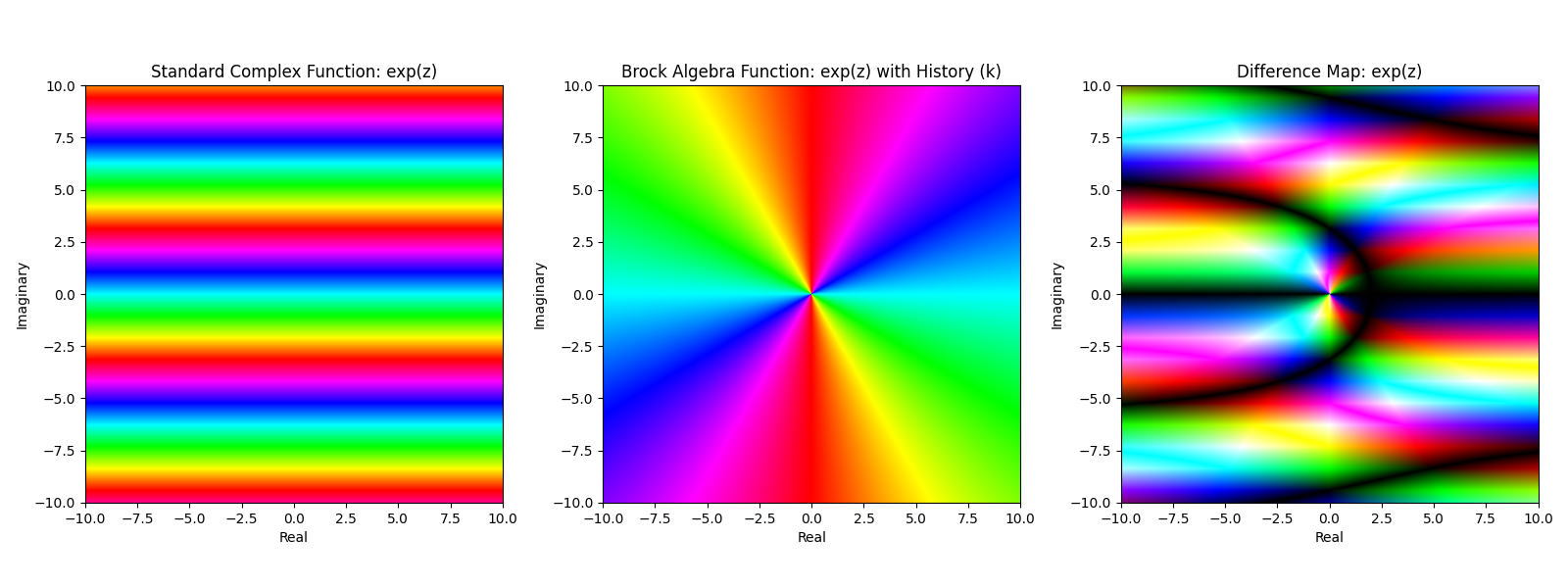
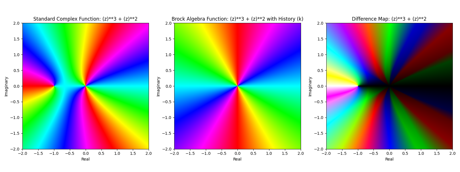
5. Illustrate with visual difference‐maps
6. Summarize conclusions and future directions

Motivation: Why Preserve Sign on Squares?

In ordinary real arithmetic, squaring a negative number loses information about the original sign. Brock Algebra seeks to maintain more of that historic data. With k₁, we intentionally keep the negative sign when a squared term originates from a negative base: This small tweak yields starkly different behaviors in composite expressions, as we’ll see.

---

Brock Algebra k-value: Tracking Sign History

Every element is encoded as a pair

(a, kₐ),    a ∈ ℝ₊,    kₐ ∈ {0, 1, …, n−1}

where

• a is the nonnegative scalar magnitude
• kₐ is the history of negative sign flips, taken modulo n

This history enables reversible operations and richer algebraic structure: each negative factor increments kₐ, and modulo wrapping prevents unbounded growth.

---

Intuition and Practical Use

• Negative multiplication as history: each “−1” factor increments kₐ by 1
• Clamped memory: (kₐ + k_b) mod n bounds history in finite cycles
• Applications: reversible transformations, provenance tracking, sign-sensitive analysis

---

Core Operations for general kₙ

1. Addition

(a, kₐ) ⊕ₙ (b, k_b) = (a + b, (kₐ + k_b) mod n)

2. Multiplication

(a, kₐ) ⊗ₙ (b, k_b) = (a · b, (kₐ + k_b) mod n)

Zero-rule: if a = 0 or b = 0 then result = (0, 0)

3. Distributivity

(a, kₐ) ⊗ₙ [ (b, k_b) ⊕ₙ (c, k_c) ]
  = ( a·(b + c),
      (kₐ + k_b + kₐ + k_c) mod n )

which equals

(a, kₐ) ⊗ₙ (b, k_b)
  ⊕ₙ
    (a, kₐ) ⊗ₙ (c, k_c)

---

Special Cases

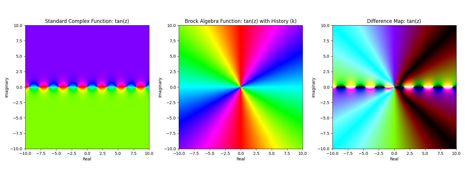
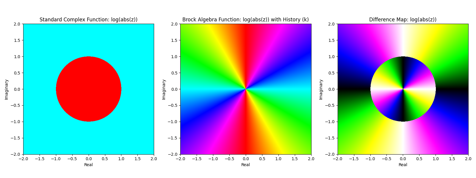
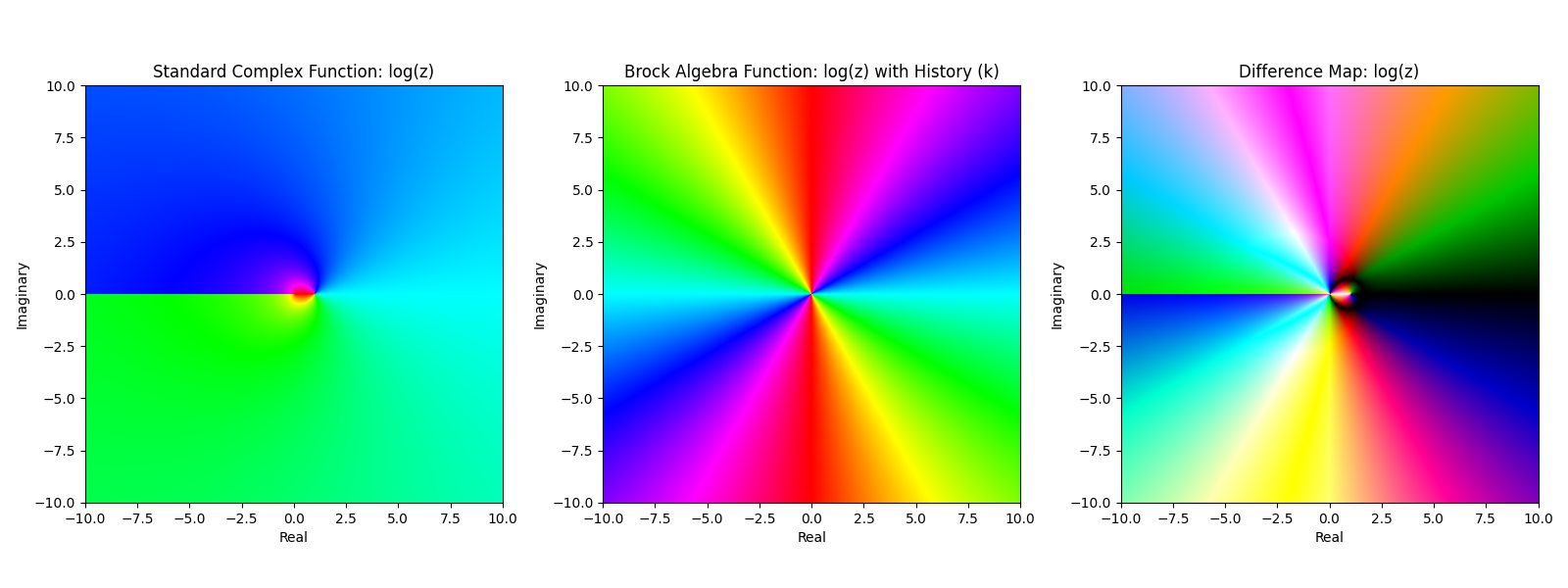
Below we demonstrate how classical, k₀, k₁, k₂, and kₙ behaviors manifest for representative functions f(x,y). For each:

1. Compute f classically
2. Compute k₀ variant on (|x|,|y|)
3. Compute k₁ variant on (|x|,|y|) with sign-history clamp
4. Compute k₂ variant on (|x|,|y|) with mod-2 toggles
5. Compute kₙ variant tracking up to n−1 flips

kₙ (general)

Preserves full cyclic memory of n sign-flips.

k₂ (mod 2): classic sign cancellation

(−1, 1) ⊗₂ (−1, 1)
  = (1, (1+1) mod 2)
  = (1, 0)

k₁ (clamped mod 1): sign-preserving clamp

Any nonzero history clamps to 1:

(a, kₐ) ⊗₁ (b, k_b)
  = (a·b, min(1, kₐ + k_b))

Examples

(2, 0) ⊗₁ (3, 0)   = (6, 0)
(−2, 1) ⊗₁ (3, 0)  = (−6, 1)
(−2, 1) ⊗₁ (−3, 1) = (6, 1)    # double negative retains k=1

k₀ (no memory): history always resets

(a, kₐ) ⊗₀ (b, k_b) = (a·b, 0)

---

Sign Representation

We encapsulate all sign information in k and keep the scalar always nonnegative. Thus any raw negative input a is encoded as:

−5 → (5, 1)
−1 → (1, 1)
 3 → (3, 0)

Example multiplications

(1, 1) ⊗ₙ (1, 0) = (1·1, (1+0) mod n) = (1, 1)
(1, 1) ⊗ₙ (1, 1) = (1·1, (1+1) mod n) = (1, 2 mod n)

In k₁, k=2 clamps to 1; in k₂, k=2 → 0; in general kₙ, k wraps mod n.

---

Conclusions and Future Directions

• k₁ uniquely preserves negativity, revealing alternating-sign phenomena
• k₂ recovers classical sign behavior
• k₀ suppresses all sign history, useful for magnitude-only workflows
• General kₙ offers tunable cyclic memory, with potential in fault-tolerant reversible computation

Brock Algebra k₁ demonstrates how a small change in exponentiation rules—preserving sign on squares—can produce complex, beautiful patterns and unlock new algebraic structures. Download our interactive notebooks and heatmap scripts to explore further, and stay tuned for deeper dives into k₂, k₃, and beyond!